Brief Intro to Numerical Methods

10/6/2026

In maths class learning calculus and differential equations the student spends most of their time finding analytic solutions to problems. Carefully chosen example problems from your friendly course instructor, are usually intended to be challenging (not-so friendly), yet possible to solve. Certain results are even perhaps elegant which exposes the student to a deeper level of understanding and intuition of the underlying mechanics of the mathematical model.

In the real world, finding exact analytical solutions to problems would be tedious and usually downright impossible. This is where future coursework in Numerical Analysis serves as a bridge between the classroom and real world industrial applications.

An early word of warning on errors, which a detailed discussion is warranted throughout the study of Numerical Analysis. In Numerical Methods we speak of solutions coupled with degrees of accuracy. In particular, in order to maintain a defined level of accuracy, it is imperative the practitioner is aware of the possible erroneous errors that may arise in the implementation of a mathematical model by a computer.

Current developments in technology has largely abstracted away the details of Numerical Methods. Yet I believe one should have a basic understanding of floating-point arithmetic. Basically, peak under the hood and ask: “how to computers really handle computations?”. As we will encounter below, being aware of of the peculiarities of computer’s floating-point operations allows us to address this potential source of error in mathematical modeling.

Review:

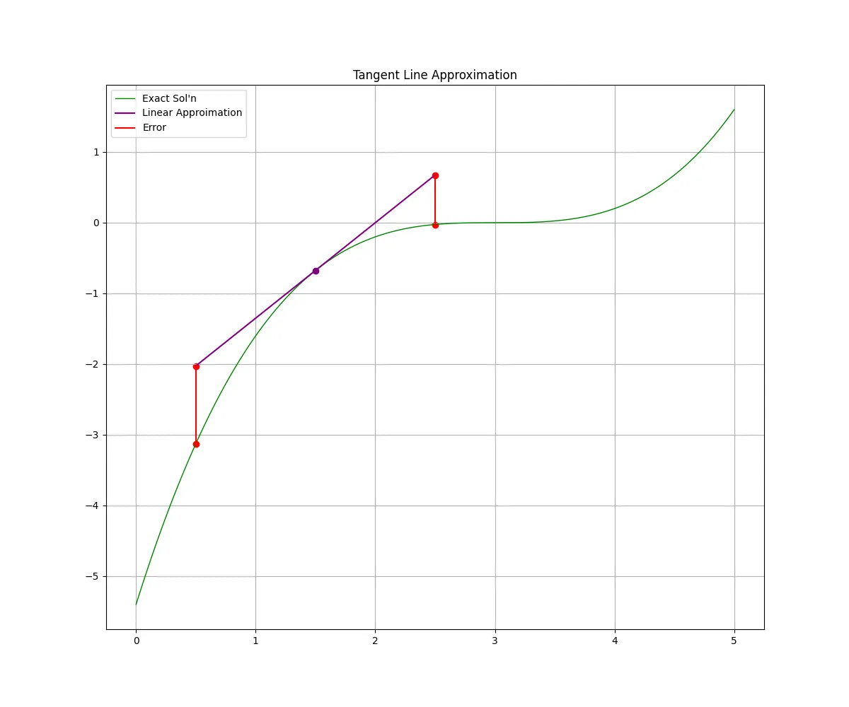
The most familiar example of Numerical Methods echos back to first-semester Calculus related to a concept called linear approximation. Given any differentiable function, we can find a (local) approximation of that function by moving in small increments along the tangent line from a known evaluated point.

Tangent Line:

$f(x_{t+1}) \approx f(x_t) + \frac{df}{dx}\left( x_t \right) (x_{t+1} - x_{t})$

To find the slope of the tangent-line in continuous calculus we take a derivative, in numerical methods we have to take a finite-difference, $\frac{\Delta f}{\Delta x}$. One of the big ideas in calculus is taking smaller and smaller step-sizes of finite-differences, we converge to the derivative. $\lim_{\Delta t \to 0}\frac{\Delta f}{\Delta x} \to \frac{df}{dx}$. We spend a fair amount of time talking about “limits” and “infinity”. In computers everything is forced to be discrete, at the lowest level, binary 1 or 0.

Approximate Accuracy

We can see that taking very tiny steps along the tangent line we remain close to the actual function $f$. Taking larger steps results in a larger error given the underlying function is non-linear about that point.

Euler’s Method:

The basic idea behind Euler’s Method is taking successive linear approximations with tiny steps, $\Delta x$, along a tangent-line, readjust your tangent line at this new point, and go again. In continuous calculus we can use Mathematical theory to let our step-sizes approach zero, our computers require discrete steps, that we can make very very small, but can’t “approach zero” in the same sense as Calculus.

Let:

$x_k := x_0 + k \cdot \Delta x$

$\tilde{f}(x_k) \approx \tilde{f}(x_{k-1}) + f'(x_{k-1}) \Delta x$

Starting with a known value, $f(x_0)$ and a tangent-slope, f’(x_0), about a point $(x_0, f(x_0))$:

• Take a tiny-step $\Delta x$
• Compute a linear approximation of $\tilde{f}(x_1)$
• Use this “guess” as the starting point for your next step: $\tilde{f}(x_{k+1})$
• Repeat

It ends up looking something like, a simple recursive pattern can be seen:

$\tilde{f}(x_1) \approx \tilde{f}(x_{0}) + f'(x_{0}) \Delta x$

$\tilde{f}(x_2) \approx \tilde{f}(x_{1}) + f'(x_{1}) \Delta x$

$\tilde{f}(x_3) \approx \tilde{f}(x_{2}) + f'(x_{2}) \Delta x$

$\tilde{f}(x_4) \approx \tilde{f}(x_{3}) + f'(x_{3}) \Delta x$

$\tilde{f}(x_5) \approx \tilde{f}(x_{4}) + f'(x_{4}) \Delta x$

$\quad \quad \quad \vdots$

$\tilde{f}(x_{n}) \approx \tilde{f}(x_{n-1}) + f'(x_{n-1}) \Delta x$

For $n$-number of discrete time-steps. $n$ could be a million if you choose. This is where the computer takes over.

Limitations:

Now if we take tiny enough step sizes, each of our approximations will be close enough to the underlying functions, with just a tiny error.

With smaller and smaller step sizes it takes more and more time to iterate over a large interval of $x$.

Say we have a tiny step-size $\Delta x := 0.00000000001$ but we are interested in $f(x)$ over a large interval, $x \in [0:100]$

Well we are going to have millions of tiny errors that accumulate by the time we reach $x=100$. The computer will also be dealing with values so small the calculations could introduce floating-point roundoff errors.

These accumulated errors will introduce drift away from the actual solution.

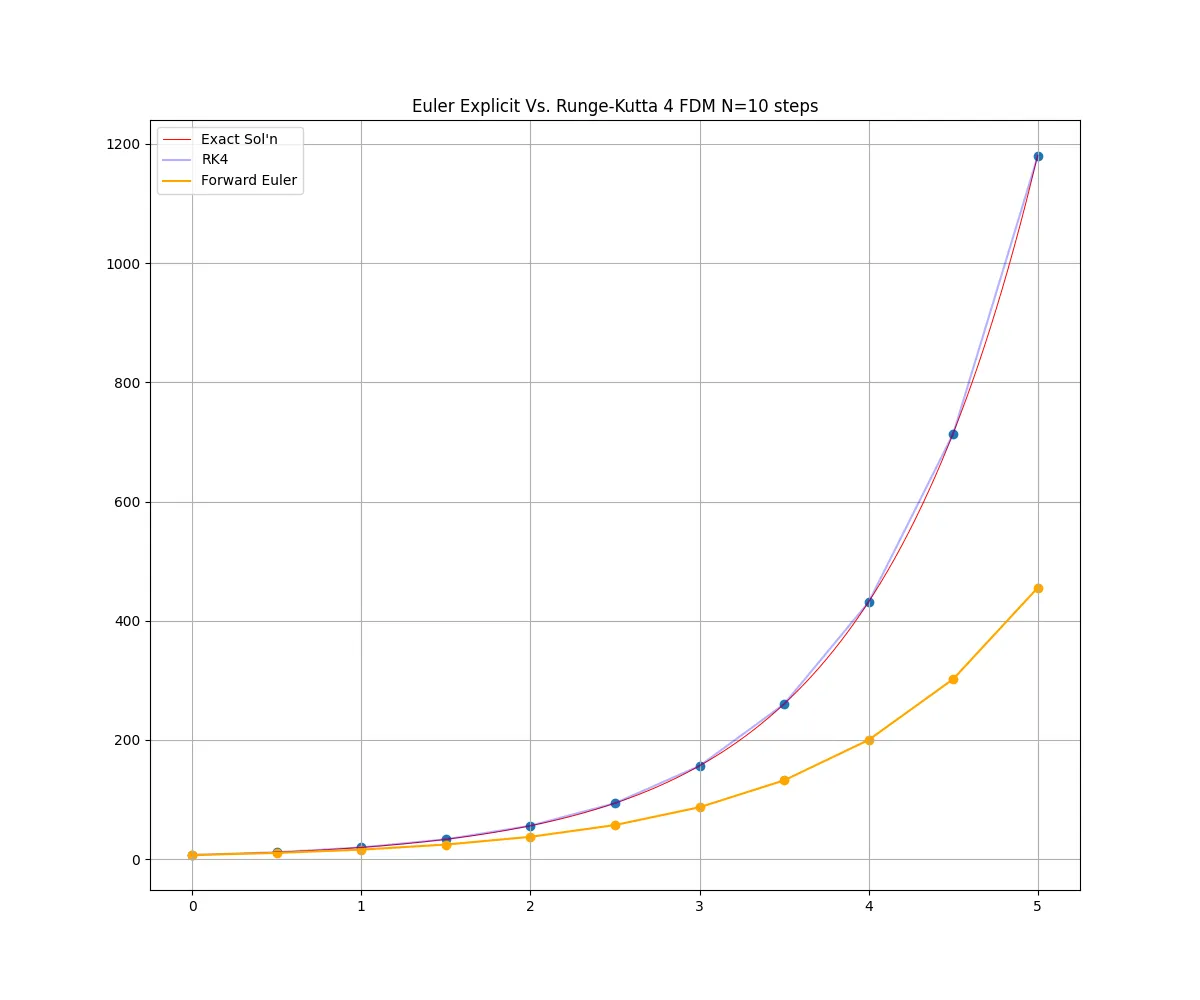
Understanding the use of Euler’s Method, and its limitations, is only a first step in Numerical Analysis. As we can see above: Runge-Kutta 4, another iterative numerical solution method, is far more accurate. Yet if you peak ‘under the hood’ of this more advanced method, it’s foundationally dependent on Euler’s Method.

Sources:

Original writing by Nicholas Alan from studying source material from Daniel Duffy, Richard Hamming, and Gilbert Strang.